Jacobian matrix of a multivariable map

For a map of multiple variables, \(F(x): \mathbb{R}^n \rightarrow \mathbb{R}^m\), its Taylor expansion at a point \(x_0\) is

\[\begin{equation} F(x) = F(x_0 + \Delta x) = F(x_0) + F_{\ast}(x_0) \Delta x + r(\Delta x), \end{equation}\]

where \(F_{\ast}(x_0)\) is the Jacobian matrix of \(F(x)\) evaluated at \(x_0\) and \(r(\Delta x)\) represents a high order residual with respect to the variable variation \(\Delta x\). The Jacobian matrix \(F_{\ast}\) captures the linear part of the map value’s variation with respect to \(\Delta x\) around \(x_0\), when \(\Delta x\) is small.

Jacobian matrix of a coordinate overlap map in differential geometry

For an \(n\)-dimensional smooth manifold, the overlap/transition map \(f_{VU}: \mathbb{R}^n \rightarrow \mathbb{R}^n\) from the coordinate chart \((U, x)\) to the chart \((V, y)\) should be a diffeomorphism, i.e. both \(f_{VU}\) and its inverse \(f_{VU}^{-1}\) are differentiable in the overlapped region \(U \cap V\). According to the inverse function theorem, if \(f_{VU}\) is a differentiable bijective map and its inverse \(f_{VU}^{-1}\) exists, the condition for \(f_{VU}^{-1}\) being continuous and differentiable in a neighborhood \(W\) of a point \(p\) in \(U \cap V\) is that the determinant of the Jacobian matrix \(\det(F_{\ast}) \neq 0\) at \(p\). If this condition holds for all \(p\) in \(U \cap V\), \(f_{VU}\) is a diffeomorphism.

The above requirement on the differentiability or smoothness of transition maps tells us coordinate charts for a manifold should not be arbitrarily selected. All charts in an atlas must conform with this smoothness structure.

Geometric meaning of the Jacobian matrix \(F_{\ast}\) for the overlap map \(f_{VU}\)

\(F_{\ast}\) transforms or pushes forward (using the terminology in differential geometry) a tangent vector represented in the chart \((U, x)\) to the representation in the chart \((V, y)\). N.B. There is only one tangent vector involved and what is transformed is its numerical representation. We can call this coordinate transformation of a physical entity. Therefore, when the determinant of the Jacobian matrix is zero, \(F_{\ast}\) is not invertible, which means it has a non-trivial kernel. For any vector in this kernel space, \(F_{\ast}\) pushes it forward to a zero tangent vector with the chart \((V,y)\). This means a local variation in \(x\) leads to no variation in \(y\); thus \(y\) cannot be locally represented with \(x\).

Take a curve embedded in a 2D plane \((x,y)\) as an example. There are two possible ways of choosing 1D coordinate chart for this curve, \(x\) or \(y\), as long as the slope at each point on this curve is a non-zero finite value. This requires each local segment of the curve should not be parallel to the \(x\) or \(y\) axis. The explicit representation of the curve equation \(y = f(x)\) is just the overlap map \(f_{yx}\). When the derivative \(\frac{\diff y}{\diff x}\) is zero at a point \(p_0 = (x_0,y_0)\) on the curve, which is the Jacobian matrix that degenerates to a scalar value, \(y\) does not change with \(x\) locally and \(y = f(x)\) does not have a local inverse.

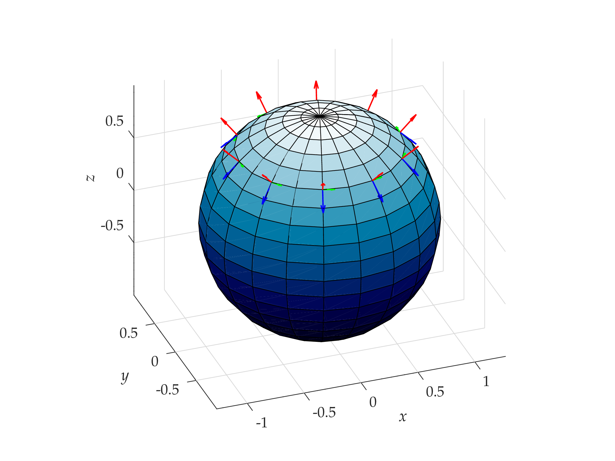
In the coordinate chart \((U, x)\), the basis vectors of the tangent space at a point \(p\) in \(U \cap V\) are \(\boldsymbol{e}_1, \cdots, \boldsymbol{e}_n\). Any \(\boldsymbol{e}_i\) can be pushed forward to the chart \((V, y)\) via \(F_{\ast}\), which is just the \(i\)-th column of \(F_{\ast}\). For example, for a unit sphere embedded in the 3D space \(\mathbb{R}^3\), the transformation from the spherical coordinates \((r, \phi, \theta)\) to Cartesian coordinates \((x, y, z)\) is

\[\begin{equation} \begin{aligned} x &= r \cos\phi \sin\theta \\ y &= r \sin\phi \sin\theta \\ z &= r \cos\theta \end{aligned}. \end{equation}\]

Its Jacobian matrix is

\[\begin{equation} \begin{pmatrix} \cos\phi \sin\theta & -r\sin\phi \sin\theta & r\cos\phi \cos\theta\\ \sin\phi \sin\theta & r\cos\phi \sin\theta & r \sin\phi \cos\theta \\ \cos\theta & 0 & -r\sin\theta \end{pmatrix}. \end{equation}\]

We can use the column vectors of this Jacobian matrix to visualize the basis vectors of the spherical coordinates in \(\mathbb{R}^3\).

Jacobian matrix of a level set

A level set is a manifold embedded in an ambient space with a higher dimension. It is usually implicitly defined as a set of constraints:

\[\begin{equation} F: \mathbb{R}^n \rightarrow \mathbb{R}^m, F(x) = y_0, x\in \mathbb{R}^n, y_0\in \mathbb{R}^m, n > m, \end{equation}\]

where \(y_0\) is a given fixed point. \(F(x) = y_0\) comprises \(m\) equations

\[\begin{equation} F(x) = \begin{cases} F^1(x) = y_0^1 \\ \quad \vdots \\ F^m(x) = y_0^m \\ \end{cases}. \end{equation}\]

The level set has \(n-m\) dimensions.

Obviously, each multivariable function \(F^i(x): \mathbb{R}^n \rightarrow \mathbb{R}\) is a 0-form defined in the ambient space \(\mathbb{R}^n\). For any given value \(y_0^i\), if \((F^i)^{-1}(y_0^i)\) is not empty, \(F^i(x) = y_0^i\) characterizes an \((n-1)\)-dimensional contour hyper-surface. The entries of the \(i\)-th row in the Jacobian matrix \(F_{\ast}\) of \(F\) are just the coefficients of the 1-form \(dF^i\):

\[\begin{equation} dF^i = \frac{\partial F^{i}}{\partial x^1} dx^1 + \cdots + \frac{\partial F^{i}}{\partial x^{n}} dx^n. \end{equation}\]

\(dF^i\) corresponds to a gradient vector rooted on the hyper-surface in the following relation

\[\begin{equation} dF^i = g \nabla F^i = \flat(\nabla F^i), \end{equation}\]

where \(g\) is the 2nd rank covariant metric tensor and \(\flat\) is the flat operator, which transforms a tangent vector to a corresponding 1-form.

Because each row in the Jacobian matrix \(F_{\ast}\) of the implicit expression for a level set defines a 1-form and this 1-form is associated with a gradient vector normal to the level set, the Jacobian matrix characterizes the normal space of the level set, which is a linear span of \(m\) 1-forms \(dF^1, \cdots, dF^m\).

The Jacobian matrix \(F_{\ast} \in \mathbb{R}^{m\times n}\) with \(n > m\) is a wide matrix. Only when \(F_{\ast}\) has a full rank in rows, i.e. \(F_{\ast}\) is a surjective map, the level set defines a manifold. This is because when \(F_{\ast}\) does not have a full rank, there exist at least two linearly dependent 1-forms, let them be \(F^i\) and \(F^j\). Because their associated gradient vectors are parallel to each other, the two level sets of \(n-1\) dimensions defined by \(F^i = y_0^i\) and \(F^j = y_0^j\) are locally tangential, which does form an effective intersection.

When \(F_{\ast}\) has a full rank in rows at a point \(p\) such that \(F(p) = y_0\), \(F_{\ast}\) is still rank deficient in its columns. So \(F_{\ast}\) is not injective at \(y_0\) and has a non-trivial kernel. This kernel is just the tangent space at \(p\) with respect to the manifold described by \(F(x) = y_0\), which annihilates the set of 1-forms \(dF^1, \cdots, dF^m\).

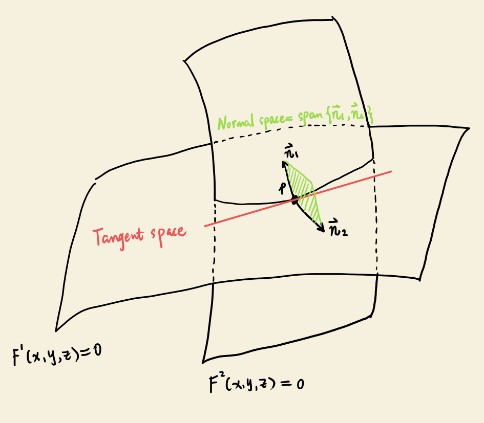
For example, let \(F: \mathbb{R}^3 \rightarrow \mathbb{R}^2\) and a one dimensional level set is implicitly defined as

\[\begin{equation} \begin{cases} F^1(x,y,z) = 0 \\ F^2(x,y,z) = 0 \end{cases}. \end{equation}\]

Let \(p\) be a point on the manifold. Then the normal space and tangent space at \(p\) are illustrated below.

Releated articles