Factor \(\sigma \) before the identity operator is always 0.5

In boundary integral equations, such as the Calderón system,

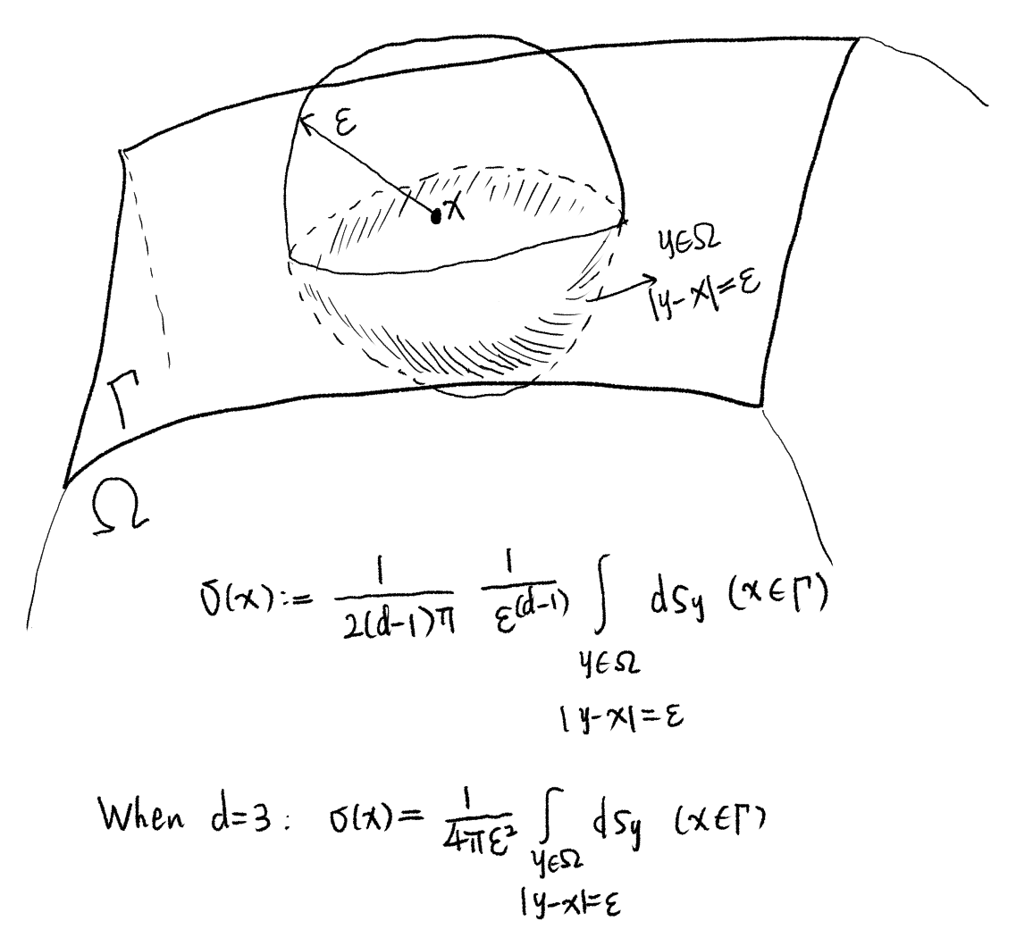
\[\begin{equation} \label{eq:bies-in-matrix-form} \begin{pmatrix} V & -K \\ K' & D \end{pmatrix} \begin{pmatrix} \tilde{t} \\ \tilde{u} \end{pmatrix} = \begin{pmatrix} \sigma I + K & -V \\ -D & (1-\sigma) I - K' \end{pmatrix} \begin{pmatrix} \tilde{g}_{\mathrm{D}} \\ \tilde{g}_{\mathrm{N}} \end{pmatrix}, \end{equation}\]

the factor \(\sigma(x)\) is defined as the solid angle of the part within \(\Omega\) of a sphere with respect to the field point \(x\in\Gamma\) divided by \(4\pi\), while the sphere is centered at \(x\):

\[\begin{equation} \sigma(x) := \lim_{\varepsilon \rightarrow 0} \frac{1}{2(d-1)\pi} \frac{1}{\varepsilon^{d-1}} \int_{y\in\Omega: \lvert y-x \rvert=\epsilon} ds_y \quad x\in\Gamma. \end{equation}\]

Therefore, \(\sigma(x)\) is the fraction of this solid angle with respect to the solid angle of the full sphere.

\(\sigma(x)\) appears in the following two cases:

1. When we take the Dirichlet trace of the double layer potential (N.B. The double layer potential is a potential generated by surface charge density and distributed in volume \(\Omega\cup\Omega^{\mathrm{c}}\)):

   \[\begin{equation} (Wv)(x) = \int_{\Gamma} \gamma_1^{\mathrm{int}}U^{\ast}(x,y) v(y) ds_y \quad x\in\Omega. \end{equation}\]

   Its interior Dirichlet trace is a potential distributed on surface

   \[\begin{equation} \gamma_0^{\mathrm{int}}(Wv)(x) = (-1 + \sigma(x)) v(x) + (Kv)(x) \quad x\in\Gamma, \end{equation}\]

   where \((Kv)(x)\) is a surface integral in the sense of Cauchy principal value, i.e. a disc centered at the field point \(x\) with a radius \(\varepsilon\) is removed from \(\Gamma\) and the remaining surface becomes the integration domain, then we evaluate the surface integral by taking the limit \(\varepsilon \rightarrow 0\).

   Its exterior Dirichlet trace is

   \[\begin{equation} \gamma_0^{\mathrm{ext}}(Wv)(x) = \sigma(x) v(x) + (Kv)(x) \quad x\in\Gamma. \end{equation}\]

   Hence the jump of the Dirichlet trace across the boundary \(\Gamma\) (defined as the exterior trace minus the interior trace, while the normal vector of \(\Gamma\) points from interior to exterior) is

   \[\begin{equation} [\gamma_0 (Wv)]_{\Gamma} = \gamma_0^{\rm ext}(Wv)(x) - \gamma_0^{\mathrm{int}}(Wv)(x) = v(x). \end{equation}\]

   The kernel function of the double layer potential in volume is the same as the kernel function of t he double layer potential boundary integral operator \(K\):

   \[\begin{equation} \gamma_1^{\mathrm{int}}U^{\ast}(x,y) = \frac{(x-y) \cdot n(y)}{4\pi \lvert x-y \rvert^3}. \end{equation}\]

   The only difference is for the kernel of \(W\), \(x\in\Omega\), while for the kernel of \(K\), \(x\in\Gamma\).

2. When we take the conormal trace or Neumann trace of the single layer potential:

   \[\begin{equation} (\tilde{V}w)(x) = \int_{\Gamma} U^{\ast}(x,y) w(y) ds_y \quad x\in\Omega. \end{equation}\]

   Its interior conormal trace is

   \[\begin{equation} \gamma_1^{\mathrm{int}}(\tilde{V}w)(x) = \sigma(x) w(x) + (K'w)(x) \quad x\in\Gamma. \end{equation}\]

   Its exterior conormal trace is

   \[\begin{equation} \gamma_1^{\mathrm{ext}}(\tilde{V}w)(x) = [\sigma(x) - 1]w(x) + (K'w)(x) \quad x\in\Gamma. \end{equation}\]

   The jump of the conormal trace across the boundary \(\Gamma\) is

   \[\begin{equation} [\gamma_1(\tilde{V}w)]_{\Gamma} = \gamma_1^{\mathrm{ext}}(\tilde{V}w)(x) - \gamma_1^{\mathrm{int}}(\tilde{V}w)(x) = -w(x) \quad x\in\Gamma. \end{equation}\]

The value of \(\sigma\) depends on the field point \(x\). When \(x\) is on a smooth surface, \(\sigma=0.5\). Obviously, when \(x\) is within a cell in a triangulation, because the cell is always a small panel approximating a local smooth surface, \(\sigma\) is also 0.5. In HierBEM, the Galerkin BEM is implemented. When we compute entries in the Galerkin matrices for \(\sigma I_1 + K_2\) and \((1-\sigma)I_2 - K_2'\), the field point \(x\) can only be one of the quadrature points in the interior of a cell \(K_x\) associated with the test space. Therefore, \(\sigma\) in Galerkin BEM is always 0.5.

If the classical collocation or Nyström method is adopted, because the collocation point may be located on an edge or at a corner, the program has to compute mesh dependent \(\sigma\). Therefore, without computing \(\sigma\) is one of the advantage of Galerkin BEM over collocation or Nyström method.