Stabilization of the hypersingular operator for the Laplace Neumann problem
Contents
2 Boundary integral equation for the Laplace problem with the Neumann boundary condition
3 Solution space of Neumann problems
3.1 Homogeneous Neumann problem
3.2 Inhomogeneous Neumann problem
4 Kernel of the hypersingular operator \(D\)
5 Select an orthogonal subspace in which the ellipticity of \(D\) holds
5.1 Choice 1: select a subspace \(L_2\)-orthogonal to natural densities
5.2 Choice 2: select a subspace \(L_2\)-orthogonal to \(\ker D\)
6 Incorporate the subspace constraint into the BIE
Abstract The hypersingular operator \(D\) appears in the boundary integral equation for the Laplace Neumann problem, which is obtained from the equation for the Neumann trace in the Caldrón system. Because \(D\) has a non-trivial kernel and lacks ellipticity on its whole domain, the solution cannot be uniquely found. Stabilization or gauging is therefore needed to modify the hypersingular operator so that the ellipticity and solution uniqueness can be restored in a subspace of \(D\)’s domain, which is orthogonal to the kernel of \(D\). Different norm or inner product definitions can be adopted to realize the said orthogonality, which lead to different solution subspaces. The final stabilized or gauged boundary integral variational equation can be obtained by enforcing the solution subspace constraint with the Lagrange multiplier method.
1 Introduction
A linear partial differential equation (PDE) or a boundary integral equation (BIE), \(Au=f\), can be analyzed in a same framework, where the solvability and stability of the equation depend on the property of the underlying linear operator \(A: X \rightarrow X'\) which maps from a Hilbert space \(X\) to its dual space \(X'\). According to the Lax-Milgram Lemma, if the linear operator is both bounded and elliptic, the solution is unique and stable. If the linear operator is not elliptic but only coercive, i.e. it satisfies a Gårdings inequality, \begin{equation} \langle (A+C)v,v \rangle \geq c_1^A \lVert v \rVert _X^2 \quad \forall v\in X, \end{equation} where \(C: X \rightarrow X'\) is a compact operator, then according to the theorem of Fredholm alternative, the solution uniqueness depends on if \(A\) is injective.
In this article, we only consider the first case above, where the Lax-Milgram Lemma and the operator’s ellipticity govern the solution property. This case is often met in both PDEs and BIEs for the Laplace problem. It is possible that the linear operator \(A\) may not be elliptic on the whole domain, such as the hypersingular boundary integral operator. Then the operator \(A\) is not invertible. Even though we can still discretize the bilinear form (in the real valued case) or sesquilinear form (in the complex valued case) \(b_A\) for \(A\), the resulted matrix \(\mathcal {A}\) will be singular and not solvable. Therefore, \(A\) should be stabilized (Steinbach) or gauged (Smirnova, b,a). Apparently, the stabilization appends additional terms to the bilinear form \(b_A\), which makes the system matrix non-singular. In essence, applying the stabilization is equivalent to searching the solution in a subspace of the operator’s domain, which is orthogonal to the kernel of the operator.
In the following, we use the BIE for the Laplace problem with the Neumann boundary condition as an example to show the mechanism of operator stabilization.
2 Boundary integral equation for the Laplace problem with the Neumann boundary condition
We usually construct a boundary integral equation by starting from the Caldrón system. If we consider an interior problem in a bounded domain \(\Omega \) in \(\mathbb {R}^d\), the Caldrón system is \begin{equation} \begin {pmatrix} \gamma _0^{\rm int} u \\ \gamma _1^{\rm int} u \end {pmatrix} = \begin {pmatrix} (1-\sigma )I-K & V \\ D & \sigma I + K' \end {pmatrix} \begin {pmatrix} \gamma _0^{\rm int} u \\ \gamma _1^{\rm int} u \end {pmatrix}. \end{equation} We organize the second row of the Caldrón system, which characterizes the Neumann trace of \(u\), and obtain the BIE for the Laplace problem with the Neumann boundary condition \(\gamma _1^{\mathrm {int}} u = g\): \begin{equation} \label {eq:op-bie-laplace-neumann} D(\gamma _0^{\mathrm {int}} u) = \left [ (1-\sigma )I-K' \right ] g. \end{equation} \(D: H^{1/2}(\Gamma ) \rightarrow H^{-1/2}(\Gamma )\) is the hypersingular boundary integral operator, which is the minus Neumann trace, i.e. conormal derivative, of the double layer potential \(Wv\), \begin{equation} (Dv)(x) = -\gamma _1^{\mathrm {int}}(Wv)(x) \quad (x\in \Gamma ), \end{equation} where \(v\) is the double layer charge density and \(v\in H^{1/2}(\Gamma )\). In the above BIE, \(v\) is just \(\gamma _0^{\mathrm {int}}u\). The integral operator \(W\) is defined as \begin{equation} \label {eq:double-layer-potential} u(x) = (Wv)(x) = \int _{\Gamma } \left ( \gamma _{1,y}^{\mathrm {int}} U^{\ast }(x,y) \right ) v(y) ds_y \quad x\in \Omega \cup \Omega ^{\mathrm {c}}, \end{equation} where \(\Omega ^{\mathrm {c}}=\mathbb {R}^d \backslash \overline {\Omega }\) and \(U^{\ast }(x,y)\) is the fundamental solution of the Laplace operator: \begin{equation} U^{\ast }(x,y) = \begin {cases} -\frac {1}{2\pi }\log \lvert x-y \rvert & \quad (d=2) \\ \frac {1}{4\pi } \frac {1}{\lvert x-y \rvert } & \quad (d=3) \end {cases}. \end{equation} \(D\) is not \(H^{1/2}(\Gamma )\)-elliptic, but only \(H^{1/2}(\Gamma )\)semi-elliptic: \begin{equation} \label {eq:hypersingular-semi-elliptic} \langle Dv,v \rangle _{\Gamma } \geq \bar {c}_1^D \lvert v \rvert _{H^{1/2}(\Gamma )}^2 \quad \forall v\in H^{1/2}(\Gamma ). \end{equation} This means the kernel of \(D\) is not trivial and the solution of the BIE in \(H^{1/2}(\Gamma )\) is not unique.
3 Solution space of Neumann problems
Before we examine the kernel of \(D\), we need several theorems about the solution space of Neumann problems from (McLean).
3.1 Homogeneous Neumann problem
Theorem 1 (Solution for the interior homogeneous Neumann problem) For the interior Laplace problem with a homogeneous Neumann boundary condition \begin{equation} \begin {cases} -\Delta u = 0 & (x\in \Omega ) \\ \gamma _1^{\rm int} u = 0 & (x\in \Gamma ) \end {cases}, \end{equation} \(u\in H^1(\Omega )\) is a solution if and only if \(u\) is constant on each disjoint component of \(\Omega \).
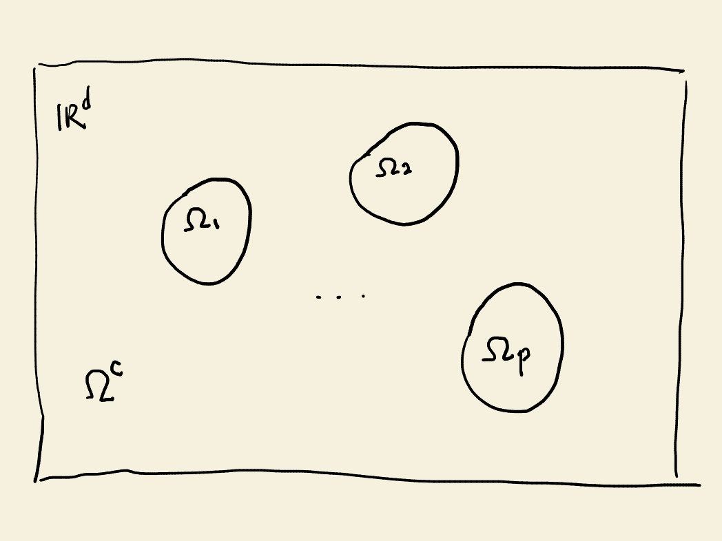
Assume \(\Omega \) comprises \(p\) components, \(\Omega _1, \cdots , \Omega _p\). Let \(v_i\) be the indicator function of \(\Omega _i\), i.e \begin{equation} v_i(x) = \begin {cases} 1 & \quad x\in \Omega _i \\ 0 & \quad x\in \Omega \backslash \Omega _i \end {cases}. \end{equation} Then \(\mathrm {span} \{ v_1,\cdots ,v_p \}\) is the solution space of the interior homogeneous Neumann problem.
Comment 1 According to the following figure, when \(\Omega =\bigcup _{i=1}^p \Omega _i\) has multiple components, we actually have \(p\) independent Neumann problems on the subdomains.
Theorem 2 (Solution for the exterior homogeneous Neumann problem) For the exterior Laplace problem with a homogeneous Neumann boundary condition \begin{equation} \begin {cases} -\Delta u = 0 & \quad (x\in \Omega ^\mathrm {c}) \\ \gamma _1^{\rm ext} u = 0 & \quad (x\in \Gamma ) \\ u(x) = O(\lvert x \rvert ^{2-d}) & \quad (\lvert x \rvert \rightarrow \infty ) \end {cases}, \end{equation} \(u\in H_{\mathrm {loc}}^1(\Omega ^{\mathrm {c}})\) is a solution if and only if it is constant on each disjoint component of \(\Omega ^{\mathrm {c}}\). When \(d\geq 3\), \(u\) attenuates to zero when \(\lvert x \rvert \rightarrow \infty \), then \(u\) is zero on the unbounded component in \(\Omega ^{\mathrm {c}}\).
Assume there are \(q\) components \(\Omega _1^{\mathrm {c}},\cdots ,\Omega _q^{\mathrm {c}}\) in \(\Omega ^{\mathrm {c}}\), where \(\Omega _q^{\mathrm {c}}\) is the unbounded domain. Let \(v_i^{\mathrm {c}}\) be the indicator function of \(\Omega _i^{\mathrm {c}}\). Then \(\mathrm {span}\{ v_1^{\mathrm {c}},\cdots ,v_{q-1}^{\mathrm {c}} \}\) is the solution space of the exterior homogeneous Neumann problem.
Comment 2 There is only one unbounded component in \(\Omega ^{\mathrm {c}}\), since if there are two such components, they intersect at the infinity, which contradicts that the components should be disjoint.
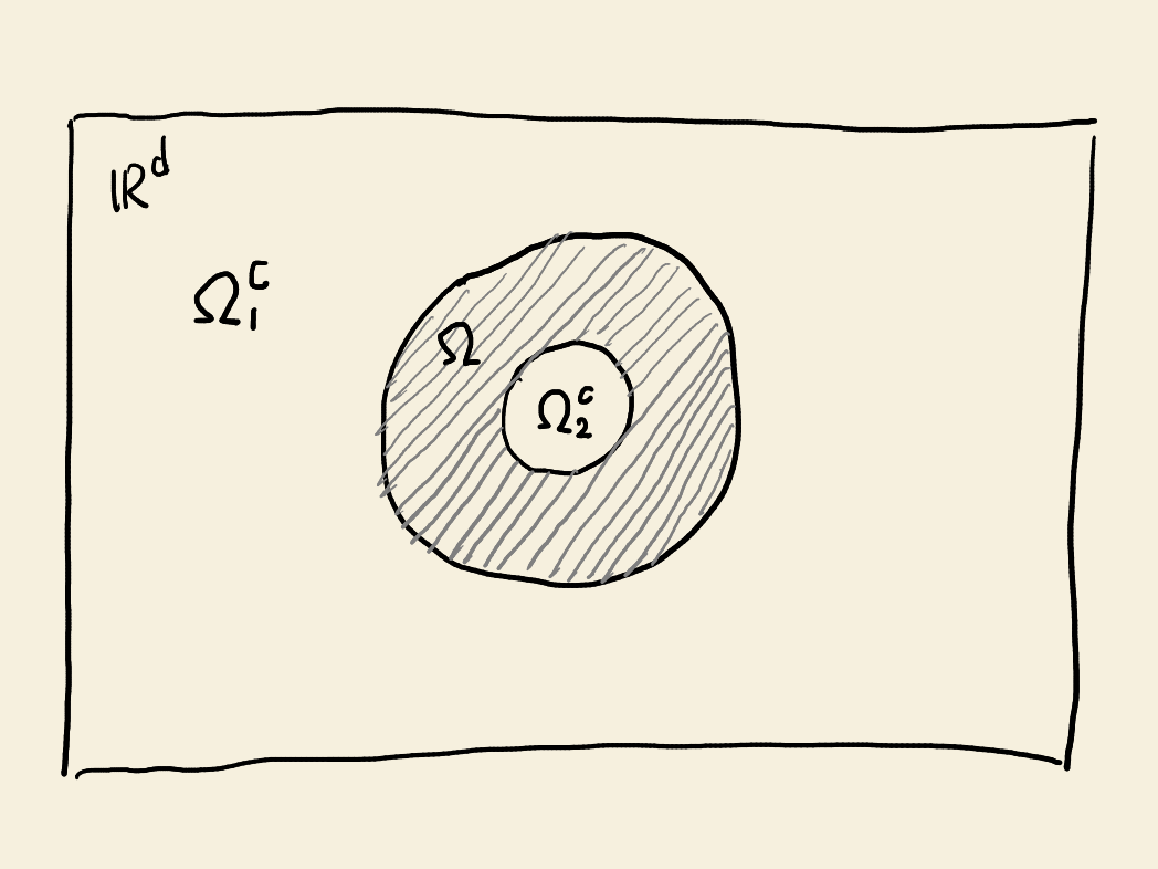
Comment 3 If the interior domain \(\Omega \) is multiply connected, the exterior domain \(\Omega ^{\mathrm {c}}\) has multiple components.
Comment 4 When the exterior domain \(\Omega ^{\mathrm {c}}\) has only one unbounded component, the solution of the exterior homogeneous Neumann problem is unique.
3.2 Inhomogeneous Neumann problem
The interior inhomogeneous Neumann problem is \begin{equation} \begin {cases} -\Delta u = f &\quad (x\in \Omega ) \\ \gamma _1^{\rm int} u=g &\quad (x\in \Gamma ) \end {cases}, \end{equation} where \(f\in \tilde {H}^{-1}(\Omega )\), \(g\in H^{-1/2}(\Gamma )\) and \(\Omega \) has \(p\) components. \(u\in H^1(\Omega )\) is a solution if and only if the solvability condition for each component \(\Omega _i\) of \(\Omega \) is satisfied \begin{equation} \int _{\Omega _i} f dx + \int _{\partial \Omega _i} g ds_x = 0 \quad 1 \leq i \leq p. \end{equation}
Comment 5 The solvability condition can be obtained from the Green’s 2nd identity, \begin{equation} \langle Lu,v \rangle _{\Omega } + \langle \gamma _1^{\mathrm {int}} u, \gamma _0^{\mathrm {int}} v \rangle _{\Gamma } = \langle Lv,u \rangle _{\Omega } + \langle \gamma _1^{\mathrm {int}} v, \gamma _0^{\mathrm {int}} u \rangle _{\Gamma }, \end{equation} by setting the test function as \(v \equiv 1\).
This indicates that if the Neumann problem can be solved with a physical meaning, the input data \(f\) and \(g\) are not independent and should not be arbitrarily given.
The solution \(u\) of the inhomogeneous Neumann problem is unique modulo the subspace \(\mathrm {span} \{ v_1,\cdots ,v_p \}\), i.e. if \(u_0\) is a solution, \(u_0 + u_1\) with \(u_1\in \mathrm {span} \{ v_1,\cdots ,v_p \}\) is also a solution. We also say the solution \(u\) is in the quotient space \(H^1(\Omega )_{/ \mathrm {span}\{ v_1,\cdots ,v_p \}}\), where all functions that have a difference within \(\mathrm {span}\{ v_1,\cdots ,v_p \}\) are considered in a same equivalence class, i.e. a solution of the inhomogeneous Neumann problem is not a single function, but a function set.
The above solution structure \(u=u_0+u_1\) is consistent with our experience acquired in the ordinary differential equation (ODE) theory, where the total solution is the sum of a particular solution for the inhomogeneous problem and a general solution for the homogeneous problem. In an ODE, the general solution is a parametric function, while in a PDE, the general solution is a function space. This also reminds us of the same solution structure for a matrix equation \(Ax=b\) in linear algebra. Such a similarity between linear algebra, ODE and PDE theories comes from the abstract linear operator theory.
The above conclusion also holds for the exterior Neumann problem.
4 Kernel of the hypersingular operator \(D\)
Theorem 3 Let \(v\in H^{1/2}(\Gamma )\) and \(Dv = 0\), then \(v\) is constant on each boundary component of \(\Gamma \). Assume \(\Gamma \) has \(r\) components, i.e. \(\Gamma = \bigcup _{i=1}^r \Gamma _i\). Let \(\chi _i\) be the indicator function for \(\Gamma _i\), then \(\mathrm {span} \{ \chi _1,\cdots ,\chi _r \}\) is the kernel of \(D\).
Proof If \(v\in H^{1/2}(\Gamma )\) is considered as the double layer charge density, the double layer potential is \begin{equation} u(x) = (Wv)(x) = \int _{\Gamma } \gamma _{1,y}^{\mathrm {int}} U^{\ast }(x,y) v(y) ds_y \quad x\in \Omega \cup \Omega ^{\mathrm {c}}. \end{equation} Because \(y\in \Gamma \) and \(x\in \Omega \cup \Omega ^\mathrm {c}\), \(x\neq y\) and there is no singularity in the above boundary integral.
Apply the Laplacian operator to the double layer potential, during which the Laplacian operator \(\Delta _x\) can be swapped with the integral operator \(\int _{\Gamma }\) since there is no singularity. \begin{equation} \begin{aligned} -\Delta _x u(x) &= -\Delta _x \int _{\Gamma } \left ( \gamma _{1,y}^{\mathrm {int}} U^{\ast }(x,y) \right ) v(y) ds_y \\ &= -\int _{\Gamma }\Delta _x \left ( \gamma _{1,y}^{\rm int} U^{\ast }(x,y) \right ) v(y) ds_y \\ &= -\int _{\Gamma } \gamma _{1,y}^{\rm int} \left ( \Delta _x U^{\ast }(x,y) \right ) v(y) ds_y \end{aligned}. \end{equation} The fundamental solution \(U^{\ast }(x,y)\) satisfies the Laplace equation with a unit Dirac source \(\delta (x-y)\): \begin{equation} -\Delta _x U^{\ast }(x,y) = \delta (x-y). \end{equation} Because \(x\neq y\), \(\delta (x-y)=0\) and \(-\Delta _x U^{\ast }(x,y) = 0\) on \(\Omega \cup \Omega ^{\mathrm {c}}\). Hence, the double layer potential \(u(x)\) is harmonic in \(\Omega \cup \Omega ^{\mathrm {c}}\).
The given condition \((Dv)(x)=0\) actually means both the interior and exterior Neumann traces of the double layer potential are zero: \begin{equation} \gamma _1^{\mathrm {int}} u = 0, \gamma _1^{\mathrm {ext}} u = 0. \end{equation} Combining these two boundary conditions with the harmonic condition \(-\Delta u = 0\) in \(\Omega \cup \Omega ^{\mathrm {c}}\), we obtain both interior and exterior homogeneous Neumann problems. According to Theorem 1 and 2, the double layer potential \(u\) must be constant on each component in \(\Omega \) and \(\Omega ^{\mathrm {c}}\). The jumping property of the double layer potential across the boundary \(\Gamma \) is \begin{equation} v(x) = [u]_{\Gamma } = \gamma _0^{\mathrm {ext}}u - \gamma _0^{\mathrm {int}}u = \lim _{\Omega ^{\mathrm {c}} \ni \tilde {x} \rightarrow x} u(\tilde {x}) - \lim _{\Omega \ni \tilde {x} \rightarrow x} u(\tilde {x}) \quad x\in \Gamma . \end{equation} This expression means the double layer charge density \(v\) at a point \(x\) on the boundary \(\Gamma \) is equal to the variation of the double layer potential \(u\), when the target point \(\tilde {x}\), which is infinitely close to \(x\), jumps across the boundary \(\Gamma \) from the interior to exterior.
Assume \(\Gamma \) has \(r\) components, \(\Gamma _1,\cdots ,\Gamma _r\). Each component \(\Gamma _i\) is shared by two components in \(\Omega \) and \(\Omega ^{\mathrm {c}}\) respectively. Then \(v\) on \(\Gamma _i\) must be constant. Therefore, the kernel of \(D\) is the span of the indicator functions of the boundary components, i.e. \(\mathrm {span} \{ \chi _1,\cdots ,\chi _r \}\). The solution of the boundary integral equation 3 is unique modulo this kernel space.
■
5 Select an orthogonal subspace in which the ellipticity of \(D\) holds
We already know that the hypersingular operator \(D\) in the BIE for the Laplace Neumann problem is not elliptic on its whole domain \(H^{1/2}(\Gamma )\), but only semi-elliptic (see Equation 7). This corresponds to the fact that the kernel of \(D\) is \(\mathrm {span} \{ \chi _1,\cdots ,\chi _r \}\) and the solution is unique only in the sense that it is an element in the quotient space \(H^{1/2}(\Gamma )_{/ \mathrm {span}\{ \chi _1,\cdots ,\chi _r \}}\). In order to make the solution authentically unique, which is mandatory for the discretized system matrix \(\mathcal {D}\) to be numerically solvable, we need to stabilize or gauge \(D\), so that it is elliptic in a subspace of \(H^{1/2}(\Gamma )\), which is orthogonal to \(\ker D\). It is in this smaller subspace that we are going to search the unique solution of the Neumann problem.
Note that the concept of orthogonality is involved here, which depends on how the inner product is defined for the Hilbert space \(H^{1/2}(\Gamma )\). Actually, we have different choices of the definitions of the inner product, which are further induced from different choices of norm definitions. If these norms are equivalent to the standard Sobolev norm of \(H^{1/2}(\Gamma )\), \(D\) must be elliptic on the subspace in which the condition of being orthogonal to \(\ker D\) holds. Therefore, the general idea to stabilize a non-elliptic operator is to select a subspace and define an equivalent norm, so that the operator is elliptic in this subspace and the subspace is orthogonal to the operator’s kernel.
5.1 Choice 1: select a subspace \(L_2\)-orthogonal to natural densities
For a boundary component \(\Gamma _i\) in \(\Gamma \) (\(i=1,\cdots ,r\)), the associated natural density \(w_{\mathrm {eq},i}\) is defined as the pre-image of the boundary indicator function \(\chi _i\) under the map of the single layer potential operator \(V\) \begin{equation} V w_{\mathrm {eq},i} = \chi _i \quad x\in \Gamma . \end{equation}
Using the standard \(L_2\) inner product1, let a subspace of \(H^{1/2}(\Gamma )\) orthogonal to these \(r\) natural densities be defined as \begin{equation} H_{\ast }^{1/2}(\Gamma ) := \{ v\in H^{1/2}(\Gamma ): \langle v,w_{\mathrm {eq},i} \rangle _{\Gamma } = 0, i=1,\cdots ,r \}. \end{equation} According to the norm equivalence of Sobolev theorem, if a norm for \(H^{1/2}(\Gamma )\) is defined as \begin{equation} \lVert v \rVert _{H_{\ast }^{1/2}(\Gamma )} := \left \{ \sum _{i=1}^r \langle v,w_{\mathrm {eq},i} \rangle _{\Gamma }^2 + \lvert v \rvert _{H^{1/2}(\Gamma )}^2 \right \}^{1/2}, \end{equation} where \(\lvert v \rvert _{H^{1/2}(\Gamma )}\) is the semi-norm of \(v\), this norm is equivalent to the Sobolev norm \(\lVert v \rVert _{H^{1/2}(\Gamma )}\) and it can be proved that \(D\) is \(H_{\ast }^{1/2}(\Gamma )\)-elliptic.
The inner product induced from this norm is \begin{equation} \langle u,v \rangle _{H_{\ast }^{1/2}(\Gamma )} := \sum _{i=1}^r \langle u,w_{\mathrm {eq},i} \rangle _{\Gamma } \langle v, w_{\mathrm {eq},i} \rangle _{\Gamma } + \lvert u \rvert _{H^{1/2}(\Gamma )} \lvert v \rvert _{H^{1/2}(\Gamma )}. \end{equation} We can verify that for any function \(v\in H_{\ast }^{1/2}(\Gamma )\), it is orthogonal to all boundary indicator functions \(\{ \chi _i \}_{i=1}^r\) using this inner product definition. \begin{equation} \langle v,\chi _i \rangle _{H_{\ast }^{1/2}(\Gamma )} = \sum _{j=1}^r \langle v,w_{\mathrm {eq},j} \rangle _{\Gamma } \langle \chi _i,w_{\mathrm {eq},j} \rangle _{\Gamma } + \lvert v \rvert _{H^{1/2}(\Gamma )} \lvert \chi _i \rvert _{H^{1/2}(\Gamma )}, \end{equation} where the sum in the above equation is zero since \(\langle v,w_{\mathrm {eq},j} \rangle _{\Gamma } = 0\) for all \(j=1,\cdots ,r\) and \(\lvert \chi _i \rvert _{H^{1/2}(\Gamma )}\) is also zero because \(\chi _i\) is constant 1 on \(\Gamma _i\) and constant 0 on other boundary components. Therefore, \(\langle v,\chi _i \rangle _{H_{\ast }^{1/2}(\Gamma )} = 0\) for all \(i=1,\cdots ,r\). Hence, \(H_{\ast }^{1/2}(\Gamma )\) is orthogonal to \(\ker D\) using the above inner product definition.
5.2 Choice 2: select a subspace \(L_2\)-orthogonal to \(\ker D\)
Using the standard \(L_2\) inner product, let a subspace of \(H^{1/2}(\Gamma )\) orthogonal to \(\ker D\), i.e. orthogonal to all boundary indicator functions \(\{ \chi _i \}_{i=1}^r\), be defined as \begin{equation} H_{\ast \ast }^{1/2}(\Gamma ) := \{ v\in H^{1/2}(\Gamma ): \langle v,\chi _i \rangle _{\Gamma } = 0, i=1,\cdots ,r \}. \end{equation} The equivalent norm for \(H^{1/2}(\Gamma )\) is defined as \begin{equation} \lVert v \rVert _{H_{\ast \ast }^{1/2}(\Gamma )} := \left \{ \sum _{i=1}^r \langle v,\chi _i \rangle _{\Gamma }^2 + \lvert v \rvert _{H^{1/2}(\Gamma )}^2 \right \}^{1/2}. \end{equation} It can be proved that \(D\) is \(H_{\ast \ast }^{1/2}(\Gamma )\)-elliptic.
The inner product induced from this norm is \begin{equation} \langle u,v \rangle _{H_{\ast \ast }^{1/2}(\Gamma )} := \sum _{i=1}^r \langle u,\chi _i \rangle _{\Gamma } \langle v,\chi _i \rangle _{\Gamma } + \lvert u \rvert _{H^{1/2}(\Gamma )} \lvert v \rvert _{H^{1/2}(\Gamma )}. \end{equation} For any function \(v\in H_{\ast \ast }^{1/2}(\Gamma )\), it is orthogonal to all boundary indicator functions \(\{ \chi _i \}_{i=1}^r\) using this inner product, i.e. for any \(i=1,\cdots ,r\), \begin{equation} \langle u,\chi _i \rangle _{H_{\ast \ast }^{1/2}(\Gamma )} = \sum _{j=1}^r \langle u,\chi _j \rangle _{\Gamma } \langle \chi _i,\chi _j \rangle _{\Gamma } + \lvert u \rvert _{H^{1/2}(\Gamma )} \lvert \chi _i \rvert _{H^{1/2}(\Gamma )} = 0. \end{equation} Therefore, \(H_{\ast \ast }^{1/2}(\Gamma )\) is orthogonal to \(\ker D\) using this new inner product definition.
6 Incorporate the subspace constraint into the BIE
In the previous section, two subspaces are constructed in which \(D\) is elliptic and the solution of the Neumann problem can be made authentically unique. So we need to incorporate these subspace constraints into the BIE for the Neumann problem. The variational formulation of the operator equation in 3 is \begin{equation} \langle D \gamma _0^{\mathrm {int}}, v \rangle _{\Gamma } = \langle [(1-\sigma )I-K']g, v \rangle _{\Gamma } \quad \forall v\in H^{1/2}(\Gamma ). \end{equation} If we restrict the solution space to \(H_{\ast }^{1/2}(\Gamma )\), we have the constrained variational formulation: for all \(v\in H_{\ast }^{1/2}(\Gamma )\), find \(\gamma _0^{\mathrm {int}}u\in H_{\ast }^{1/2}(\Gamma )\), such that \begin{equation} \begin{aligned} \langle D \gamma _0^{\mathrm {int}}u,v \rangle _{\Gamma } &= \langle [(1-\sigma )I-K']g, v \rangle _{\Gamma } \\ \langle \gamma _0^{\rm int}u, w_{\mathrm {eq},i} \rangle _{\Gamma } &= 0 \quad i=1,\cdots ,r \end{aligned}. \end{equation} Using the Lagrange multiplier method, we obtain a saddle point problem: for all \(v\in H^{1/2}(\Gamma )\), find \(\gamma _0^{\mathrm {int}}u \in H^{1/2}(\Gamma )\), such that \begin{equation} \begin{aligned} \langle D \gamma _0^{\rm int}u,v \rangle _{\Gamma } + \sum _{i=1}^r \lambda _i \langle v,w_{\mathrm {eq},i} \rangle _{\Gamma } &= \langle [(1-\sigma )I-K']g, v \rangle _{\Gamma } \\ \langle \gamma _0^{\rm int}u, w_{\mathrm {eq},i} \rangle _{\Gamma } &= 0 \quad i=1,\cdots ,r \end{aligned}, \end{equation} where \(\lambda _1,\cdots ,\lambda _r\) are Lagrange multipliers2.
Because the above test function \(v\) is arbitrary in \(H^{1/2}(\Gamma )\), we can select \(v\) as a boundary indicator function \(\chi _i\). Because \(D\) is self-adjoint and \(\chi _i\) belongs to \(\ker D\), we have \begin{equation} \langle D \gamma _0^{\mathrm {int}}u,v \rangle _{\Gamma } = \langle D \gamma _0^{\mathrm {int}}u,\chi _i \rangle _{\Gamma } = \langle \gamma _0^{\mathrm {int}}u, D\chi _i \rangle _{\Gamma } = 0. \end{equation} Meanwhile, according to the closed range theorem, \(\mathrm {Im} D = ( \ker D' )^{\circ } = ( \ker D )^{\circ }\), where \(( \ker D )^{\circ }\) is the annihilator of \(\ker D\). Because \([(1-\sigma )I-K']g\) in the right hand side term belongs to the image of \(D\), it also belongs to \(( \ker D )^{\circ }\), so we have \begin{equation} \langle [(1-\sigma )I-K']g,\chi _i \rangle _{\Gamma } = 0. \end{equation} Therefore, the first equation in the above saddle point problem becomes \begin{equation} \sum _{j=1}^r \lambda _j \langle \chi _i, w_{\mathrm {eq},j} \rangle _{\Gamma } = 0. \end{equation} Because \(\langle \chi _i, w_{\mathrm {eq},j} \rangle _{\Gamma }\) cannot be ensured to be zero, all the Lagrange multipliers \(\lambda _1,\cdots ,\lambda _r\) must be zero. Then we can introduce a factor \(\alpha \in \mathbb {R}^+\) to obtain an equivalent saddle point problem as below. \begin{equation} \begin{aligned} \langle D \gamma _0^{\rm int}u,v \rangle _{\Gamma } + \sum _{i=1}^r \lambda _i \langle v,w_{\mathrm {eq},i} \rangle _{\Gamma } &= \langle [(1-\sigma )I-K']g, v \rangle _{\Gamma } \\ \langle \gamma _0^{\rm int}u, w_{\mathrm {eq},i} \rangle _{\Gamma } - \frac {\lambda _i}{\alpha } &= 0 \quad i=1,\cdots ,r \end{aligned}. \end{equation} The Lagrange multiplier can be represented as \begin{equation} \lambda _i = \alpha \langle \gamma _0^{\mathrm {int}}u, w_{\mathrm {eq},i} \rangle _{\Gamma }. \end{equation} Substitute this expression into the first equation, we obtain the stabilized variational equation for the Neumann problem: for all \(v\in H^{1/2}(\Gamma )\), find \(\gamma _0^{\mathrm {int}}u\in H^{1/2}(\Gamma )\), such that \begin{equation} \langle D \gamma _0^{\mathrm {int}}u,v \rangle _{\Gamma } + \alpha \sum _{i=1}^r \langle \gamma _0^{\mathrm {int}}u, w_{\mathrm {eq},i} \rangle _{\Gamma } \langle v,w_{\mathrm {eq},i} \rangle _{\Gamma } = \langle [(1-\sigma )I-K']g,v \rangle _{\Gamma }. \end{equation} The left hand side of this equation can be considered as a stabilized bilinear form \(\langle \tilde {D}\gamma _0^{\mathrm {int}}u, v \rangle _{\Gamma }\), which is \(H^{1/2}(\Gamma )\)-elliptic. Therefore, the solution of this equation is unique and is ensured to be in the subspace \(H_{\ast }^{1/2}(\Gamma )\).
If we restrict the solution to the subspace \(H_{\ast \ast }^{1/2}(\Gamma )\), using the Lagrange multiplier method, we obtain a new saddle point problem: for all \(v\in H^{1/2}(\Gamma )\), find \(\gamma _0^{\mathrm {int}}u \in H^{1/2}(\Gamma )\), such that \begin{equation} \begin{aligned} \langle D \gamma _0^{\rm int}u,v \rangle _{\Gamma } + \sum _{i=1}^r \lambda _i \langle v,\chi _i \rangle _{\Gamma } &= \langle [(1-\sigma )I-K']g, v \rangle _{\Gamma } \\ \langle \gamma _0^{\rm int}u, \chi _i \rangle _{\Gamma } &= 0 \quad i=1,\cdots ,r \end{aligned}. \end{equation} Again, that all Lagrange multipliers \(\lambda _1,\cdots ,\lambda _r\) are zero can be deduced from the first equation. Introducing another factor \(\bar {\alpha }\in \mathbb {R}^+\), we obtain the second formulation of the stabilized variational equation for the Neumann problem: for all \(v\in H^{1/2}(\Gamma )\), find \(\gamma _0^{\mathrm {int}}u\in H^{1/2}(\Gamma )\), such that \begin{equation} \langle D \gamma _0^{\mathrm {int}}u,v \rangle _{\Gamma } + \alpha \sum _{i=1}^r \langle \gamma _0^{\mathrm {int}}u, \chi _i \rangle _{\Gamma } \langle v,\chi _i \rangle _{\Gamma } = \langle [(1-\sigma )I-K']g,v \rangle _{\Gamma }. \end{equation} The left hand side of this equation is a stabilized bilinear form \(\langle \hat {D}\gamma _0^{\mathrm {int}}u, v \rangle _{\Gamma }\), which is also \(H^{1/2}(\Gamma )\)-elliptic. The solution of this equation is unique and is ensured to be in the subspace \(H_{\ast \ast }^{1/2}(\Gamma )\).
References
William Charles Hector McLean. Strongly Elliptic Systems and Boundary Integral Equations. Cambridge University Press. ISBN 978-0-521-66375-5.
Yulia Smirnova. Calderon preconditioning for higher order boundary element method, a.
Yulia Smirnova. Dual mesh calderon preconditioning for single layer boundary integral operator, b.
Olaf Steinbach. Numerical Approximation Methods for Elliptic Boundary Value Problems: Finite and Boundary Elements. Springer Science & Business Media. ISBN 978-0-387-31312-2.
1Actually, because \(v\) and \(w_{\mathrm {eq},i}\) belong to two spaces dual to each other, the \(L_2\) inner product used here is actually duality pairing.
2We should be careful here: while \(\gamma _0^{\mathrm {int}}u\) appears in the subspace constraint \(\langle \gamma _0^{\mathrm {int}}u, w_{\mathrm {eq},i} \rangle _{\Gamma } = 0\), \(v\) instead of \(\gamma _0^{\mathrm {int}}u\) appears in the Lagrange multiplier term \(\lambda _i\langle v,w_{\mathrm {eq},i} \rangle _{\Gamma }\) in the first equation, even though it is related to the constraint for \(\gamma _0^{\mathrm {int}}u\).
Backlinks: 《Evaluation of the stabilization term for the hypersingular operator》