Plot a figure with LaTeX symbols in Octave
Adding LaTeX equations to a figure is very useful for mathematical visualization. Unlike MATLAB which has a simple tex interpreter for typesetting text labels, Octave itself does not support rendering math equations. However, by cooperating with LaTeX, Ghostscript and epstopdf, Octave can handle this task with professional quality, which is much better than MATLAB. This is achieved by the epslatexstandalone driver provided in the print function.
I adopt the following procedure to produce figures with different formats depending on the file’s extension name.
- Plot the figure and print it using the
epslatexstandalonedriver. It generates an EPS file as well as a tex file that includes this EPS file. - Use
sedto inject a line of LaTeX code which imports my own LaTeX template. - Compile the LaTeX file into a dvi file.
- Convert the dvi file to an EPS file.
- Use Ghostscript or
epstopdfcommand to transform the EPS file to the final target.
I’ve written a script PrintGCFLatex to automate the above process.
function PrintGCFLatex(varargin)
  ## PrintGCFLatex - Print the current figure with text processed by LaTeX. The
  ## resulted file is generated in the current directory.

  [reg, prop] = parseparams(varargin);

  ## Take the first number valued argument as the figure handle. If
  ## not specified, use the current figure.
  if (length(reg) > 0)
    h = reg{1};
  else
    h = gcf;
  endif

  if (length(prop) > 0)
    ## Take the first string argument as the figure file name.
    filename = prop{1};
    if (length(prop) > 1)
      resolution = prop{2};
    else
      resolution = 500;
    endif
  else
    error("Please provide the figure file name!");
  endif

  ## Get the extension of the figure file name.
  [dir_name, base_name, ext_name] = fileparts(filename);

  if (isempty(ext_name))
    ext_name = ".png";
  endif

  tex_name = cstrcat(base_name, ".tex");
  dvi_name = cstrcat(base_name, ".dvi");
  eps_name = cstrcat(base_name, ".eps");

  ## Generate an eps figure with text processed by LaTeX.
  print(h, eps_name, "-depslatexstandalone");
  ## Use sed to insert my own LaTeX template into the tex file.
  system(cstrcat("sed -i '4i \\\\\\input{octave-plot}' ", "\"", tex_name, "\""));
  ## Process the tex file and generate dvi file.
  system(cstrcat("latex ", "\"", tex_name, "\""));
  ## Convert the dvi file to eps file.
  system(cstrcat("dvips -E ", "\"", dvi_name, "\"", " -o ", "\"", eps_name, "\""));

  ## Convert the eps file to other formats using Ghostscript.
  switch(ext_name)
    case ".jpg"
      system(cstrcat("gs -dNOSAFER ", "-r", num2str(resolution), " -dBATCH -sDEVICE=jpeg -dNOPAUSE -dEPSCrop -sOutputFile=", "\"", cstrcat(base_name, ".jpg"), "\" ", "\"", eps_name, "\""));
    case ".png"
      ## Use device png256 instead of pngalpha, which has better visualization effect.
      system(cstrcat("gs -dNOSAFER ", "-r", num2str(resolution), " -dBATCH -sDEVICE=png256 -dNOPAUSE -dEPSCrop -sOutputFile=", "\"", cstrcat(base_name, ".png"), "\" ", "\"", eps_name, "\""));
    case ".pdf"
      system(cstrcat("epstopdf ", eps_name));
    otherwise
      error("Figure format not implemented!");
  endswitch
endfunction
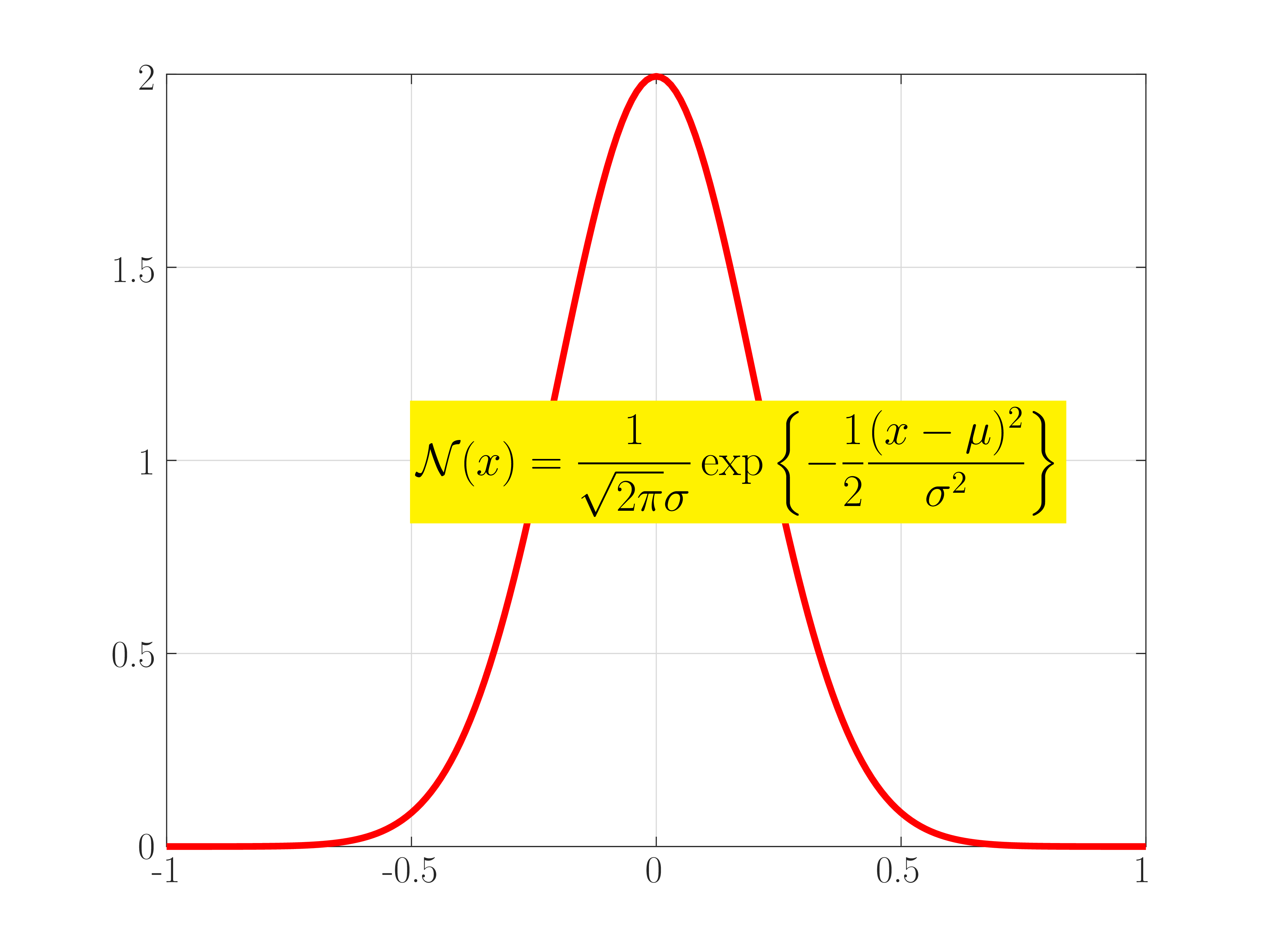
Now, let’s plot a Gaussian function as an example, where the LaTeX equation is placed in a colored box.
cd "./figures";
x = -1:0.01:1;
y = gaussian_distribution(x, 0, 0.2^2);
figure(1, "visible", "off");
plot(x, y, 'r-', "linewidth", 3);
text(-0.5, 1, "\\colorbox{yellow}{$\\displaystyle{\\mathcal{N}(x) = \\frac{1}{\\sqrt{2\\pi}\\sigma} \\exp\\left\\{ -\\frac{1}{2} \\frac{(x-\\mu)^2}{\\sigma^{2}} \\right\\}}$}", "fontsize", 20);
set(gca, "fontsize", 18);
grid on;
PrintGCFLatex("2022-11-26-gaussian.png");
ans = "./figures/2022-11-26-gaussian.png";